 EN
EN DE
DE ES
ES FR
FR PT
PT IT
IT


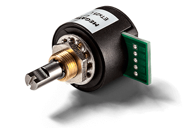
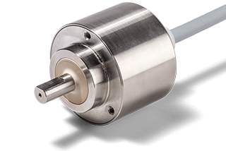
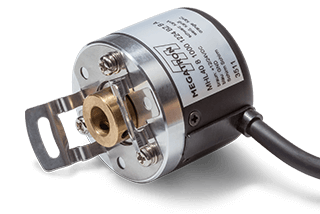
Incremental Encoders
Optical and magnetic encoders with incremental output
Guide Incremental Encoders
Index
What is an incremental encoder?
Incremental encoders are rotary encoders that provide an output signal in the form of pulses. One pulse corresponds to one period, the increment, after which this type of encoder is named. Incremental encoders are also called rotary pulse encoders because of their characteristics as encoders for rotary motion and their signal form. The use of pulses for measurement is a fundamentally different principle from, for example, potentiometers and absolute encoders.
The most important property for determining the angular accuracy of an incremental encoder is the number of pulses generated per full revolution of the shaft at the output (pulses per revolution, ppr.). This value can be found on any incremental encoder datasheet.

An external evaluation unit, such as a counter, is always required to evaluate signals from incremental encoders.
- If the angle is to be recorded, the number of pulses must be counted by an evaluation unit. If the angle is to be recorded, the information from the increments must be evaluated. For example, if the incremental encoder delivers 360 ppr, then 1° corresponds to exactly one pulse.
- For an angular velocity measurement (angle change per time unit), the number of pulses per time unit is calculated
In general, there are some things to consider when evaluating the signals, see Signal Evaluation of Incremental Signals.
Operating Principles
There are several sensor principles that can be used to implement incremental encoders. The most common is probably optoelectronic detection, which is used in optical encoders. Another possibility is magnetic sensing. Hall encoders are also available with incremental outputs. MEGATRON only uses modern gradient based Hall sensors.
Optical incremental encoders
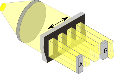
The figure shows a simplified illustration of the imaging measurement principle of an optical encoder. The two detectors A and B are illuminated with a spatial offset during the rotation of the coding wheel (black), generating pulses.
Optical sensor technology has several advantages that make optical encoders the most important incremental encoders. Firstly, the fact that the measuring method of the integrated sensor elements itself generates increments, and therefore the use in incremental encoders is obvious. An overview of optical encoders can be found here.
The optical system of a modern optical incremental encoder consists of at least the following components:
- A light-emitting diode (LED) that produces light
- A collimator that directs the light from the LED in parallel
- A coding wheel having alternating permeable and non-permeable (or reflective and absorptive) regions
- The photodetector, which detects the incident light from the LED and converts it into an electrical signal.
Two methods have become established on the market: The transmissive (imaging) method and the reflective (interferential) method. In the transmissive method, the coding wheel is transilluminated, whereas in the reflective method, the light beam is reflected from the surface of the coding wheel and interference effects are used.
A brief explanation of the transmissive method:
The light is collimated (parallelized) and passed through the coding wheel. The wheel ensures that light and dark areas on the detectors alternate periodically. The signal from the two photodetectors is normally 90° out of phase. As a result, the direction of rotation can be determined from the sequence of the signals or their spacing in the output signal.
The structure varies according to the requirements. For example, additional elements in the design of the sensor generate a reference pulse that only generates a signal on a third channel once per revolution. This reference allows the absolute angle to be calculated. This means that the number of pulses is counted from the reference. If the count is lost due to a power interruption, the reference angle can be used to recover the absolute angle information.
Coding wheels for optical encoders
Coding wheels are made from a variety of materials, usually metal, glass or plastic. Plastic is mainly used for low-cost encoders. Metal coding wheels are very robust. Comparing metal with glass or plastic, it is not possible to achieve such high optical resolutions with the same diameter using the transmissive method. With the reflective method, the incremental structure is printed on the coding wheel and it is possible to achieve finer structures.
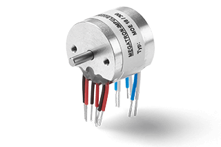
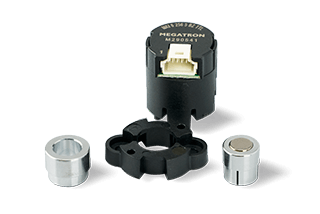
Hall effect incremental encoders
Hall encoders are also available with incremental outputs. As with optical encoders, the measurement technology is contactless and therefore virtually wear-free (apart from the bearing). The main advantages of Hall effect incremental encoders are the virtually unlimited life of the sensor technology (no ageing of the LEDs) and excellent shock resistance. Disadvantages can be the sensitivity to external interference and the fact that the signals are transmitted with a slight time delay (update rate). For an explanation of the measuring principle of Hall-effect encoders, see the guide to absolute encoders guide. For a more detailed analysis of the advantages and disadvantages of different encoder technologies, see the rotary encoder guide.
Signal evaluation of incremental signals
Channels, resolution and direction of rotation
Incremental encoders usually have several signal outputs. If an incremental encoder outputs several signal packages, the term channel is used in this context. For example "Channel A" and "Channel B". In the literature, the term "track" is also used instead of "channel".
Example:
If the data sheet of an incremental encoder specifies the value 360 ppr and the encoder has the electrical signal outputs "A" and "B" ("Channel A" and "Channel B"), then 360 pulses per one revolution of the shaft (per 360°) are output at output "A" and another 360 ppr 90° ahead or behind the pulses of channel A are output at output "B". In total, the encoder generates 720 ppr per full shaft revolution (360°) for both channels A and B.
The number of pulses per revolution (ppr) is also referred to as the resolution, the higher the value ppr), the higher the angular resolution of the encoder.

The square wave signals of "Channel B" are either 90° ahead or 90° behind the signals of "Channel A". Whether the "Channel A" signal is 90° ahead or 90° behind the "Channel B" signal depends on the product and is specified in the data sheet. In most cases, there is an illustration of the signal output function in conjunction with the direction of rotation indication, showing the signal sequence of the channels.
Example:
In the illustration on the right, CW (clockwise) is defined as the direction of rotation. When the encoder is viewed from the front (with the shaft end of the encoder facing the viewer) and the encoder shaft is rotated clockwise, the output of the "Channel B" signal is delayed by 90° relative to the output of "Channel A". However, if the shaft is rotated counter-clockwise, the signal from "Channel B" will be 90° ahead of the signal from "Channel A".
This relationship can be used in an evaluation unit to detect the direction of rotation. The number of pulses, pulse length and period of track A and track B are identical. When exchanging an encoder for another model, these characteristics are decisive, as the programming of the evaluation unit does not need to be changed if the signal sequences of the products to be exchanged are identical.
Z-track / Index Signal
Often an additional track can be selected as an option, the so-called index track or "Z-track". The Z-track output provides an index signal in the form of a single square pulse for each full shaft revolution (360°).
The index signal has two main functions:
- As a zero reference: After a voltage-free period, the index pulse can be used to move to a defined zero point.
- As a reference pulse: Particularly for encoders operating at very high speeds, the reference pulse has a control function as a separate count pulse for a full stroke/revolution.
Case study:
A check is made to see if the number of 'normal' counted pulses between two consecutive index pulses matches the expected number. For example, if an encoder with a specification of 16000 pulses/revolution is used and the evaluation unit counts less than 16000 pulses per full revolution, an error has occurred.
Edge evaluation / quadrature signal
The 90° signal offset of the square wave signals of channels A and B has an advantage. For each track and signal period, a square-wave signal has one rising and one falling signal edge.
The edge sequence for tracks A and B of a signal period is as follows:
Track A rising edge (1) → after a ¼ period Track B rising edge (2) → after a ½ period Track A falling edge (3) → after a ¾ period Track B falling edge (4)
If an evaluation unit evaluates not only the rising edge of one track, but also the rising and falling edges of both tracks A and B, then the number of pulses can be quadrupled using this method. This is equivalent to a fourfold increase in accuracy without any structural changes to the encoder.

Example:
If the incremental encoder datasheet specifies a resolution of 1024 ppr, this would be four times higher with edge evaluation, i.e. 4096 signals per revolution per channel. The edge evaluation just described is also called "quadrature signal with directional information". An edge evaluation can be based, for example, on the integrated circuit LS7083 offered by MEGATRON.
Maximum speed and cut-off frequency
Incremental encoders cannot be operated at any speed. There are mechanical and/or electronic limitations.
The mechanical limitations can be determined from the data sheet and are due to the following causes:
- Max. shaft bearing speed (only applies to encoders with their own shaft bearing, see Shaft encoders). The maximum allowable speed is often less than 10000 rpm.
- The eccentricity (unbalance) of the mechanics. With optical encoders, this is mainly caused by the imbalance of the coding wheel. However, the maximum operating speed can be as high as 60,000 rpm. Magnetic kit encoders, on the other hand, do not normally have this limitation.
The electronic limitation can be calculated: here the result of the calculation is called the "theoretical maximum possible actuating speed".
- The reason for this is the cut-off frequency of the electronics. The electronics cannot process a frequency higher than the cut-off frequency. The higher the cut-off frequency and the lower the resolution of the encoder, the higher is the theoretically possible actuating speed.
The following formula can be used to calculate the theoretical maximum actuating speed from the cut-off frequency:
\(max. rpm =\frac{\text {cut-off frequency} \frac {1} {s} * 60 }{ \text {number of pulses}}\)

Two examples of how to calculate the theoretical maximum actuating speed are given below.
Example 1:
A resolution of 512 ppr is required. The cut-off frequency is given as 100 kHz in the encoder datasheet. You get
\({100000 \cdot 1/s\cdot 60 \text{ s} \over 512} = 11718 \text { rpm} \)
Result: The theoretical maximum permissible actuating speed is 11718 rpm.
Example 2:
The required resolution is 10000 ppr. The cut-off frequency is specified as 100 kHz in the encoder datasheet. Result: The theoretical maximum actuating speed of the actuator is 600 rpm.
\({100000 \cdot 1/s \cdot 60 \text{ s} \over 10000} = 600 \text { rpm} \)
A comparison between the maximum theoretical and mechanically permissible actuation speed shows which one counts for the application: the lower of the two values is relevant!
Tolerances and deviations of optical incremental encoders
No incremental encoder provides a perfect signal. For optical incremental encoders, the following describes the uncertainties or tolerances that must be considered for the signals from these encoders. The optical system includes the encoder wheel itself and the encoder module or assembly containing the LED and photodetector. All these elements interact to produce some deviation from the ideal rectangular signal shape and ideal edge position. These tolerances are often described in the datasheet of an optical incremental encoder and help the user to analyse the measurement data more accurately.
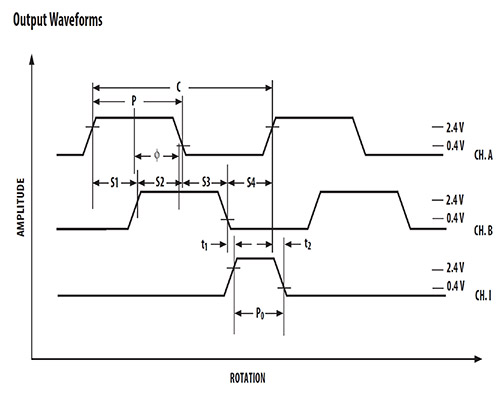
In most cases, the signals from channels A, B and, if necessary, Z are shown as a picture. The relationships are then explained using examples in the diagram opposite.
The symbols have the following meanings:
C corresponds to a period
P stands for a ½ signal period
S for ¼ Signal period
Ф is the phase reference between channels A and B
In the ideal case: C = 2 * P = 4 * S = S1 + S2 + S3 + S4.
Example for describing the tolerance field of a quarter period duration
One increment, and therefore one period, ideally consists of four equidistant signal components (C/4). Since in practice a signal period is not divided into four equal parts, the possible ratio and thus the tolerance band of the four parts of a signal period (T) to each other is described. The following term describes that a quarter of the signal period can vary by a twelfth of the signal period:
\(S1,S2,S3,S4 = \frac {C} {4} \pm \frac {C} {12}\)
Example of a half-period tolerance field description
One increment, and therefore one signal period, ideally consists of two equidistant signal components (C/2). Since a signal period does not always consist of exactly two wave pairs of equal length, the possible ratio of the two wave pairs of a signal period (T) to each other is described. The following term describes that half a period or half a signal period or half a wavelength can vary by plus/minus one twelfth of the ideal.
\(P = \frac {C} {2} \pm \frac {C} {12}\)
Description of the possible phase shift between channel A and B
Ideally, the phase shift between channel A and B is exactly 90° (ninety degrees). The 90° are shown in the relationship C/4. So a quarter of a signal period corresponds to 90°. The error in this case can be ± C/24, i.e. plus-minus one twenty-fourth. One twenty-fourth corresponds to 360°/24, which corresponds to a possible phase error of plus-minus 15°. Thus, the relationship of the increments between channels A and B can be in a range of 90° ±15° and the phase reference between channels A and B can be in a range of 75°...105°.
\(Ф = \frac {C} {4} \pm \frac {C} {24}\)
Description of the index pulse length tolerance band (channel Z)
The index pulse is output once every 360° when the shaft is driven continuously in one direction. One period corresponds to C. The representation C/4 means that the index pulse is ideally ¼ the length of one signal period. The pulse width of the index pulse can deviate from the ideal, i.e. the length of a quarter signal period (=C/4), by plus/minus one twelfth of a signal period.
This means that the pulse width of the index pulse can vary between 1/3 (=C/3) and 1/6 (=C/6) of a signal period.
\(Po = \frac {C} {4} \pm \frac {C} {12}\)
Sine/Cosine Interpolation
The more pulses per revolution that are realised with an optical encoder, the smaller the line width of the increments on the code wheel. However, the optical system of an angle encoder can only detect increments up to a certain line width. For example, a 10 mm diameter code wheel cannot have 10,000 lines due to its small size. When incremental encoders with a small housing diameter and high resolution are to be implemented, this is often done on the basis of sine/cosine interpolation.
In this method, the encoder's optical system is not used as in a conventional optical incremental encoder, so that there are abrupt changes in state between transmission and transmission interruption, or reflection and reflection interruption. Instead, the transition between zero and maximum transmission or reflection is as smooth as possible. The smooth transition results in a sinusoidal function of the signal. A second LED and phototransistor are required to produce a cosine signal. The sine and cosine signals are then digitized. A continuous sampling rate is usually used.
Example:
If a coding wheel is used from which 8 sine periods are obtained, this corresponds to a resolution of 3 bits. However, if this sine signal is sampled with 10 bits, the (digitization) resolution is 213 bits, which is equivalent to a resolution of 8192 ppr. The advantage of the principle is therefore obvious.
Optical and magnetic encoders with analogue output are also available, providing sine and cosine analogue signals. With such an encoder, subsequent interpolation is possible.
Output interfaces
The characteristics of incremental signals (high-low, on-off, Boolean logic) make them particularly suitable for use in digital circuits. Many incremental encoder series therefore offer interfaces that allow easy integration into such circuit networks:
- OC (Open Collector)
- Standard voltage output or TTL (transistor transistor logic)
- PP (Push Pull)
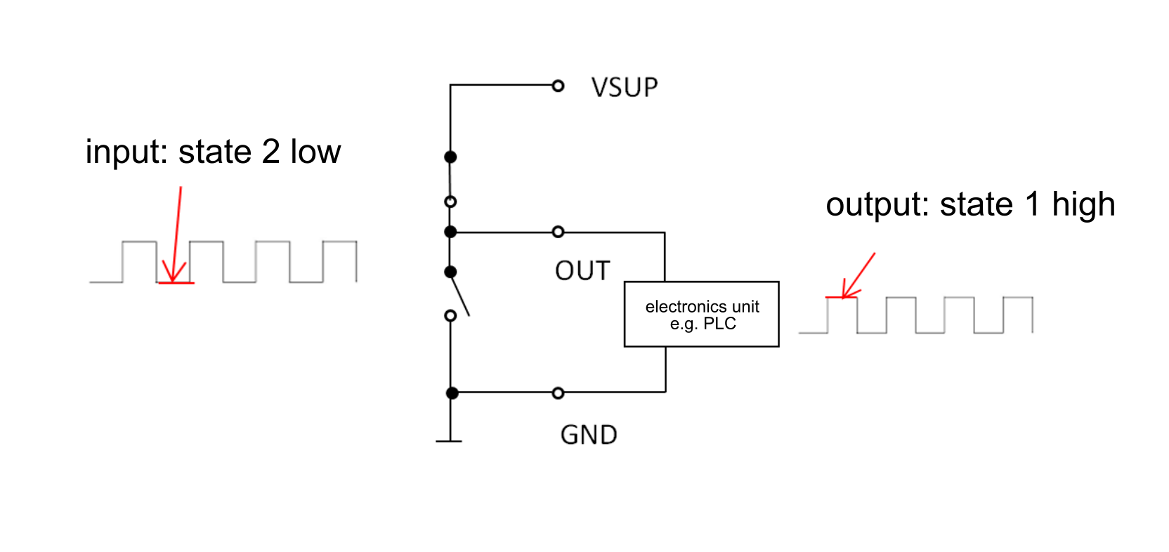
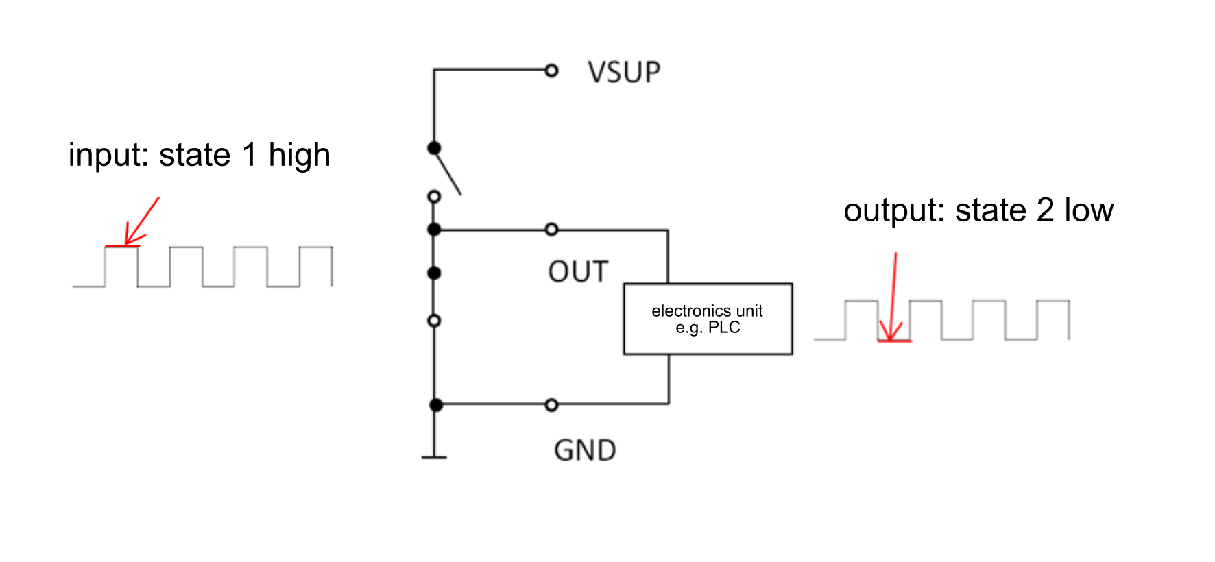
Open Collector (OC) Output
The open collector circuit is an obvious standard for output circuits for incremental signals, and a major advantage is that it allows the output to be connected to a different voltage level defined by the application. This is possible because there is no pull-up resistor integrated into the encoder and the collector is led out of the housing (open collector). The transistor thus acts as a switch.
The following example applies to a bipolar Si-NPN transistor:
High level at signal output:
- A low level (<0.7V) at the base of the transistor blocks the transistor and the supply voltage (VSUP) is applied to the collector.
Low level at the signal output:
- When the base of the transistor is high (>0.7V), the voltage at the collector (VSUP) is pulled to ground.

With the open collector circuit it is usually necessary to connect a pull-up resistor between the supply voltage and the signal outputs A, B and Z of the encoder (collector). This ensures that the levels can be detected by the evaluation unit as low and high levels. A typical value for a pull-up resistor can be 4.7 kOhm. The maximum collector voltage depends on the transistor used and is usually specified in the encoder datasheet. Since it exceeds 50 V, incremental signals with very high signal levels can be transmitted over long distances. Due to the variability of the collector voltage, level conversion is also possible.
TTL output
The TTL output is often simply referred to as the voltage output. The difference to the open collector output is that the necessary pull-up resistors are already integrated in the encoder housing, so the levels are fixed. Variable level conversion as with the open collector circuit is therefore not possible.
These levels are for standard TTL logic:
< 0.4 V for the low level
> 2.4 V for the high level

Push / Pull output
The push/pull output circuit is based on a complementary pair of transistors (n-channel and p-channel). It alternately blocks one of the two transistors.
When the output signal is high, it is at the level of VSUP and when it is low, it is approximately at ground. The advantage of a push-pull circuit is that no additional pull-up or pull-down resistors are required. If no level conversion is required, encoders with push-pull output circuitry can be used as a universal replacement for open collector and TTL/voltage outputs.

Low level at the transistor inputs: NPN disables and PNP opens
High level is VSUP
High level at the transistor inputs: NPN opens and PNP disables
Level Low approximately to ground


Incremental encoders are used wherever angles, speeds or angular velocities need to be measured with high accuracy. Incremental encoders provide output signals in the form of pulses, which are counted by an external evaluation unit. The sensors of the high-quality products used by MEGATRON are based on non-contact measuring principles, such as optoelectronic and magnetic (Hall effect) sensor technology.
Optical incremental encoders are insensitive to external interference and offer the highest precision for positioning or adjustment operations. Magnetic encoders are extremely durable and highly resistant to vibration. With a wide range of designs and output options available, there is an incremental encoder to suit almost any application.
However, special applications often require technical adaptations, which we at MEGATRON can make even for relatively small quantities. Our aim is to offer each customer the best functional and economical product for their application. As a reliable partner, we support you from the enquiry stage through to the start of series production and right up to the end of the product life cycle with high delivery reliability and quality assurance.